• On each node, a decision tree asks a question and answers it with yes/no to classify observations under that node.
• The question could be based on a specific True/False (is obs.feature = something) question or could be based on numeric data (is obs.feature > 10)
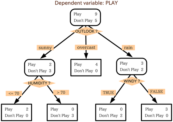
• The classification can be categorical or numerical
• The first node is called the Root node, the nodes in the middle are called internal nodes, and the results are called leaf nodes

# source https://scikit-learn.org/stable/modules/tree.html#classification
from sklearn import tree
from sklearn.datasets import load_iris
from sklearn import tree
import pandas as pd

iris = load_iris()
X, y = load_iris(return_X_y=True)
X_df = pd.DataFrame(X, columns=iris.feature_names)
X_df.head()

	sepal length (cm)	sepal width (cm)	petal length (cm)	petal width (cm)
0	5.1	3.5	1.4	0.2
1	4.9	3.0	1.4	0.2
2	4.7	3.2	1.3	0.2
3	4.6	3.1	1.5	0.2
4	5.0	3.6	1.4	0.2

# Imagine we need to pick a root node ourselves: we'll need to see how each feature performs on the split
## Fitting our tree on the train data
import matplotlib.pyplot as plt

for feature in iris.feature_names:
  plt.figure(figsize=(10,6))
  clf = tree.DecisionTreeClassifier(max_depth=1)
  clf = clf.fit(X_df.loc[:,feature].values.reshape(-1,1), y)
  print("Decision tree based on {0}".format(feature))
  tree.plot_tree(clf, filled=False, impurity=False) 
  plt.show()

Decision tree based on sepal length (cm)

Decision tree based on sepal width (cm)

Decision tree based on petal length (cm)

Decision tree based on petal width (cm)

• When the leaves don't contain 100% of our data, we consider them "impure"
• Now, to get our Root node, we'll need to measure this "impurity" concept and choose the "best" feature as a root
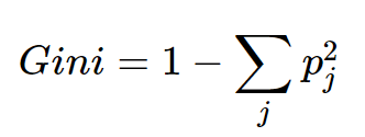
• The most popular way to measure impurity is Gini (more on it here interpretation and intuitive explanation of Gini impurity )

• So now, based on this impurity measure we can evaluate what the best split is (all we'll to do is calculate the weighted average for the leaf nodes of each split)

# This process is already implemented in the sklearn library. 
## So let's look at what it yields!
clf = tree.DecisionTreeClassifier()
plt.figure(figsize=(20,10))
tree.plot_tree(clf.fit(X, y), impurity=True, feature_names=iris.feature_names) 
plt.show()

## Plotting the tree (alternative - useful when tree is big!)
import graphviz 
dot_data = tree.export_graphviz(clf, out_file=None) 
graph = graphviz.Source(dot_data) 
graph.render("iris")

dot_data = tree.export_graphviz(clf, out_file=None, 
                     feature_names=iris.feature_names,  
                     class_names=iris.target_names,  
                     filled=True, rounded=True,  
                     special_characters=True)  
graph = graphviz.Source(dot_data)  
graph 

# see also: plot Decision surface of a decision tree using paired features
# https://scikit-learn.org/stable/auto_examples/tree/plot_iris_dtc.html